tagtango

Input data requirements

tagtango is flexible in handling various data types. To date, it accepts input in the form of either a MultiAssayExperiment R object stored as an RDS file (Ramos et. al., 2017), a SingleCellExperiment R object stored as an RDS file (Amezquita et. al., 2020), or an R data frame stored as an RDS, CSV, or TSV file.

`MultiAssayExperiment` object

Providing a MultiAssayExperiment object as input will allow you to study multiple data modalities simultaneously. However, there are certain criteria that needs to be met. First, the elements of the ExperimentList container should be SingleCellExperiment following the specifications stated in the next section. Second, cells in all elements of the ExperimentList should be the same (and have unique and matching names). Finally, different annotations should be stored as columns of the colData data frame within the object.

As test dataset, a preprocessed and annotated 10x dataset is provided with the package. This is a MultiAssayExperiment with Peripheral Blood Mononuclear Cells (PBMCs) from a healthy donor stained with a few TotalSeq-B antibodies (10x Genomics, 2018), and is readily accessible via:

library(tagtango)
data(test_data)
test_data

## A MultiAssayExperiment object of 2 listed
##  experiments with user-defined names and respective classes.
##  Containing an

## ExperimentList class object of length 2:
##  [1] RNA: SingleCellExperiment with 33538 rows and 7472 columns
##  [2] ADT: SingleCellExperiment with 17 rows and 7472 columns
## Functionality:
##  experiments() - obtain the ExperimentList instance
##  colData() - the primary/phenotype DataFrame
##  sampleMap() - the sample coordination DataFrame
##  `$`, `[`, `[[` - extract colData columns, subset, or experiment
##  *Format() - convert into a long or wide DataFrame
##  assays() - convert ExperimentList to a SimpleList of matrices
##  exportClass() - save data to flat files

Notice that the column and row names of each SingleCellExperiment in the corresponding ExperimentList object are not NULL, and that the different annotations are stored in:

MultiAssayExperiment::colData(test_data)

## DataFrame with 7472 rows and 21 columns
##                                    Sample            Barcode       sum
##                               <character>        <character> <numeric>
## AAACCCAAGATTGTGA-1 /var/folders/w9/2_9f.. AAACCCAAGATTGTGA-1      6160
## AAACCCACATCGGTTA-1 /var/folders/w9/2_9f.. AAACCCACATCGGTTA-1      6713
## AAACCCAGTACCGCGT-1 /var/folders/w9/2_9f.. AAACCCAGTACCGCGT-1      3637
## AAACCCAGTATCGAAA-1 /var/folders/w9/2_9f.. AAACCCAGTATCGAAA-1      1244
## AAACCCAGTCGTCATA-1 /var/folders/w9/2_9f.. AAACCCAGTCGTCATA-1      2611
## ...                                   ...                ...       ...
## TTTGTTGGTTCAAGTC-1 /var/folders/w9/2_9f.. TTTGTTGGTTCAAGTC-1      5830
## TTTGTTGGTTGCATGT-1 /var/folders/w9/2_9f.. TTTGTTGGTTGCATGT-1      4096
## TTTGTTGGTTGCGGCT-1 /var/folders/w9/2_9f.. TTTGTTGGTTGCGGCT-1      5524
## TTTGTTGTCGAGTGAG-1 /var/folders/w9/2_9f.. TTTGTTGTCGAGTGAG-1      4039
## TTTGTTGTCGTTCAGA-1 /var/folders/w9/2_9f.. TTTGTTGTCGTTCAGA-1      4213
##                     detected subsets_Mito_sum subsets_Mito_detected
##                    <integer>        <numeric>             <integer>
## AAACCCAAGATTGTGA-1      2194              523                    11
## AAACCCACATCGGTTA-1      2093              415                    11
## AAACCCAGTACCGCGT-1      1518              287                    11
## AAACCCAGTATCGAAA-1       737              110                    12
## AAACCCAGTCGTCATA-1      1240              156                    11
## ...                      ...              ...                   ...
## TTTGTTGGTTCAAGTC-1      2178              323                    11
## TTTGTTGGTTGCATGT-1      1256              256                    11
## TTTGTTGGTTGCGGCT-1      1907              574                    11
## TTTGTTGTCGAGTGAG-1      1605              271                    10
## TTTGTTGTCGTTCAGA-1      1549              209                    11
##                    subsets_Mito_percent altexps_Antibody.Capture_sum
##                               <numeric>                    <numeric>
## AAACCCAAGATTGTGA-1              8.49026                          981
## AAACCCACATCGGTTA-1              6.18203                         1475
## AAACCCAGTACCGCGT-1              7.89112                         7149
## AAACCCAGTATCGAAA-1              8.84244                         6831
## AAACCCAGTCGTCATA-1              5.97472                         6839
## ...                                 ...                          ...
## TTTGTTGGTTCAAGTC-1              5.54031                         9520
## TTTGTTGGTTGCATGT-1              6.25000                         7763
## TTTGTTGGTTGCGGCT-1             10.39102                         1973
## TTTGTTGTCGAGTGAG-1              6.70958                         4316
## TTTGTTGTCGTTCAGA-1              4.96084                         5682
##                    altexps_Antibody.Capture_detected
##                                            <integer>
## AAACCCAAGATTGTGA-1                                17
## AAACCCACATCGGTTA-1                                17
## AAACCCAGTACCGCGT-1                                17
## AAACCCAGTATCGAAA-1                                17
## AAACCCAGTCGTCATA-1                                17
## ...                                              ...
## TTTGTTGGTTCAAGTC-1                                17
## TTTGTTGGTTGCATGT-1                                17
## TTTGTTGGTTGCGGCT-1                                17
## TTTGTTGTCGAGTGAG-1                                17
## TTTGTTGTCGTTCAGA-1                                16
##                    altexps_Antibody.Capture_percent     total sizeFactor
##                                           <numeric> <numeric>  <numeric>
## AAACCCAAGATTGTGA-1                          13.7376      7141   1.301038
## AAACCCACATCGGTTA-1                          18.0142      8188   1.417836
## AAACCCAGTACCGCGT-1                          66.2804     10786   0.768162
## AAACCCAGTATCGAAA-1                          84.5944      8075   0.262742
## AAACCCAGTCGTCATA-1                          72.3704      9450   0.551463
## ...                                             ...       ...        ...
## TTTGTTGGTTCAAGTC-1                          62.0195     15350   1.231340
## TTTGTTGGTTGCATGT-1                          65.4608     11859   0.865106
## TTTGTTGGTTGCGGCT-1                          26.3172      7497   1.166710
## TTTGTTGTCGAGTGAG-1                          51.6577      8355   0.853067
## TTTGTTGTCGTTCAGA-1                          57.4229      9895   0.889817
##                       Main.ADT    Fine.ADT RNA.Azimuth.L1 RNA.Azimuth.L2
##                    <character> <character>    <character>    <character>
## AAACCCAAGATTGTGA-1   cluster 2   cluster 9           Mono      CD14 Mono
## AAACCCACATCGGTTA-1   cluster 2   cluster 3           Mono      CD14 Mono
## AAACCCAGTACCGCGT-1   cluster 2   cluster 3           Mono      CD14 Mono
## AAACCCAGTATCGAAA-1   cluster 5   cluster 4             NK             NK
## AAACCCAGTCGTCATA-1   cluster 5   cluster 4             NK             NK
## ...                        ...         ...            ...            ...
## TTTGTTGGTTCAAGTC-1   cluster 5   cluster 4              B B intermediate
## TTTGTTGGTTGCATGT-1   cluster 8   cluster 8          CD8 T      CD8 Naive
## TTTGTTGGTTGCGGCT-1   cluster 2   cluster 3           Mono      CD14 Mono
## TTTGTTGTCGAGTGAG-1   cluster 4   cluster 6        other T           MAIT
## TTTGTTGTCGTTCAGA-1   cluster 4   cluster 6          CD4 T        CD4 TCM
##                           RNA.Azimuth.L3 RNA.singleR.L1 RNA.singleR.L2
##                              <character>    <character>    <character>
## AAACCCAAGATTGTGA-1             CD14 Mono      Monocytes      Monocytes
## AAACCCACATCGGTTA-1             CD14 Mono      Monocytes      Monocytes
## AAACCCAGTACCGCGT-1             CD14 Mono      Monocytes      Monocytes
## AAACCCAGTATCGAAA-1                  NK_1       NK cells       NK cells
## AAACCCAGTCGTCATA-1                  NK_1       NK cells       NK cells
## ...                                  ...            ...            ...
## TTTGTTGGTTCAAGTC-1 B intermediate lambda       NK cells       NK cells
## TTTGTTGGTTGCATGT-1             CD8 Naive   CD8+ T-cells   CD8+ T-cells
## TTTGTTGGTTGCGGCT-1             CD14 Mono      Monocytes      Monocytes
## TTTGTTGTCGAGTGAG-1                  MAIT   CD8+ T-cells       CD4+ Tem
## TTTGTTGTCGTTCAGA-1             CD4 TCM_1   CD4+ T-cells       CD4+ Tcm
##                    ADT.citesort    ADT.citesort.rename
##                     <character>            <character>
## AAACCCAAGATTGTGA-1     147_leaf CD45RO- CD16- monocyte
## AAACCCACATCGGTTA-1     151_leaf CD45RA+ CD56+ CD16- ..
## AAACCCAGTACCGCGT-1     125_leaf CD45RA+ CD45RO- CD16..
## AAACCCAGTATCGAAA-1      63_leaf    CD16+ CD56+ NK cell
## AAACCCAGTCGTCATA-1      63_leaf    CD16+ CD56+ NK cell
## ...                         ...                    ...
## TTTGTTGGTTCAAGTC-1      38_leaf CD16+ CD56+ TIGIT+ B..
## TTTGTTGGTTGCATGT-1      23_leaf      naive CD8+ T cell
## TTTGTTGGTTGCGGCT-1      67_leaf CD45RA+ CD45RO- CD16..
## TTTGTTGTCGAGTGAG-1     169_leaf central memory CD4+ ..
## TTTGTTGTCGTTCAGA-1     159_leaf central memory CD4+ ..

`SingleCellExperiment` object

Providing a SingleCellExperiment object, one also needs to ensure that the data is formatted in a specific manner. First, data should be normalized and stored as a logcounts assay within the SingleCellExperiment object. For example, in the main text, CITE-seq data was normalized using the R package ADTnorm. Second, cell and marker names within the SingleCellExperiment object should be defined (ensure these are not set as NULL). Finally, different annotations should be stored as columns of the colData within the object. Likewise, the object can contain the principal components of the data calculated using different decomposition techniques in reducedDims (see Amezquita et. al. 2020 for further information). Notice that an example of a SingleCellExperiment that can be used as input by tagtango can be generated using:

test_data[["ADT"]]

## class: SingleCellExperiment 
## dim: 17 7472 
## metadata(1): Samples
## assays(1): logcounts
## rownames(17): CD3 CD4 ... IgG1 IgG2b
## rowData names(3): ID Symbol Type
## colnames(7472): AAACCCAAGATTGTGA-1 AAACCCACATCGGTTA-1 ...
##   TTTGTTGTCGAGTGAG-1 TTTGTTGTCGTTCAGA-1
## colData names(20): Sample Barcode ... RNA.singleR.L2 ADT.citesort
## reducedDimNames(1): UMAP
## mainExpName: ADT
## altExpNames(0):

Data frame object

Providing a data frame object is the simplest way to run tagtango. The application expects different annotations to be stored as columns of the data frame. An example of a data frame that can be used as input by tagtango can be generated again with:

MultiAssayExperiment::colData(test_data)

Supplementary usage scenario: comparing spatial transcriptomics annotations

To highlight the versatility of tagtango, we tested our software on a different data modality. We used an annotated spatial transcriptomics dataset provided as part of the spatialLIBD project (Maynard et. al., 2021;, Pardo et. al., 2022). The data was generated with 10x Genomics Visium platform and contain human brain tissue samples from three healthy donors. In particular, these are spatially adjacent replicates of human dorsolateral prefrontal cortex tissue. This dataset is interesting because it investigates the laminar structure of the brain cortex, providing several manual annotations of the different layers for the individual spots (considered as `ground truth’) as well as several cluster-based annotations.

Following the input data requirements outlined above, we prepared the dataset with R to be studied with tagtango. First, we followed Pardo et. al., (2022), and downloaded the spatial transcriptomics dataset.

# Load libraries
library(spatialLIBD)
library(SingleCellExperiment)
library(scater)

# Download data
spe <- fetch_data(type = "spe")

The data comes in the form of a SpatialExperiment R object. We reshaped the data into a SingleCellExperiment object using

sce <- SingleCellExperiment(
        list( logcounts = logcounts(spe) ),
        colData = cbind( colData(spe), spatialCoords(spe) ),
        rowData = rowData(spe)
     )
    
sce <- runUMAP(sce, exprs_values = "logcounts")

Notice that the spatial coordinates of the spatial transcriptomics dataset were added as columns in the colData object (these could also be added as part of the reducedDims object), and that we calculated the UMAP decomposition using the R package scater (McCarthy et. al., 2017).

Finally, this object contains multiple samples for a spatial transcriptomics dataset; therefore, the column names are not unique. Likewise, row names (i.e. gene IDs) can also be more intuitive if we use the gene names as opposed to ensembl names. To fix this, we used:

# Row names
rownames(sce) <- rowData(sce)$gene_name

# Fix col names (they were not unique)
colnames(sce) <- rownames(data.frame(colData(sce)))

Using tagtango, we then compared sets of annotations for this dataset. A first interesting comparison is that between the consensus manual annotations and one of the best performing unsupervised clustering method used in (Maynard et. al., 2021). In particular, we focused on the differences between ‘ground truth’ annotations and annotations using highly variable genes from scran (Lun et. al., 2016), 50 PCs for dimension reduction, and spatial coordinates as features (i.e. method HVG\_PCA\_spatial as described in Maynard et. 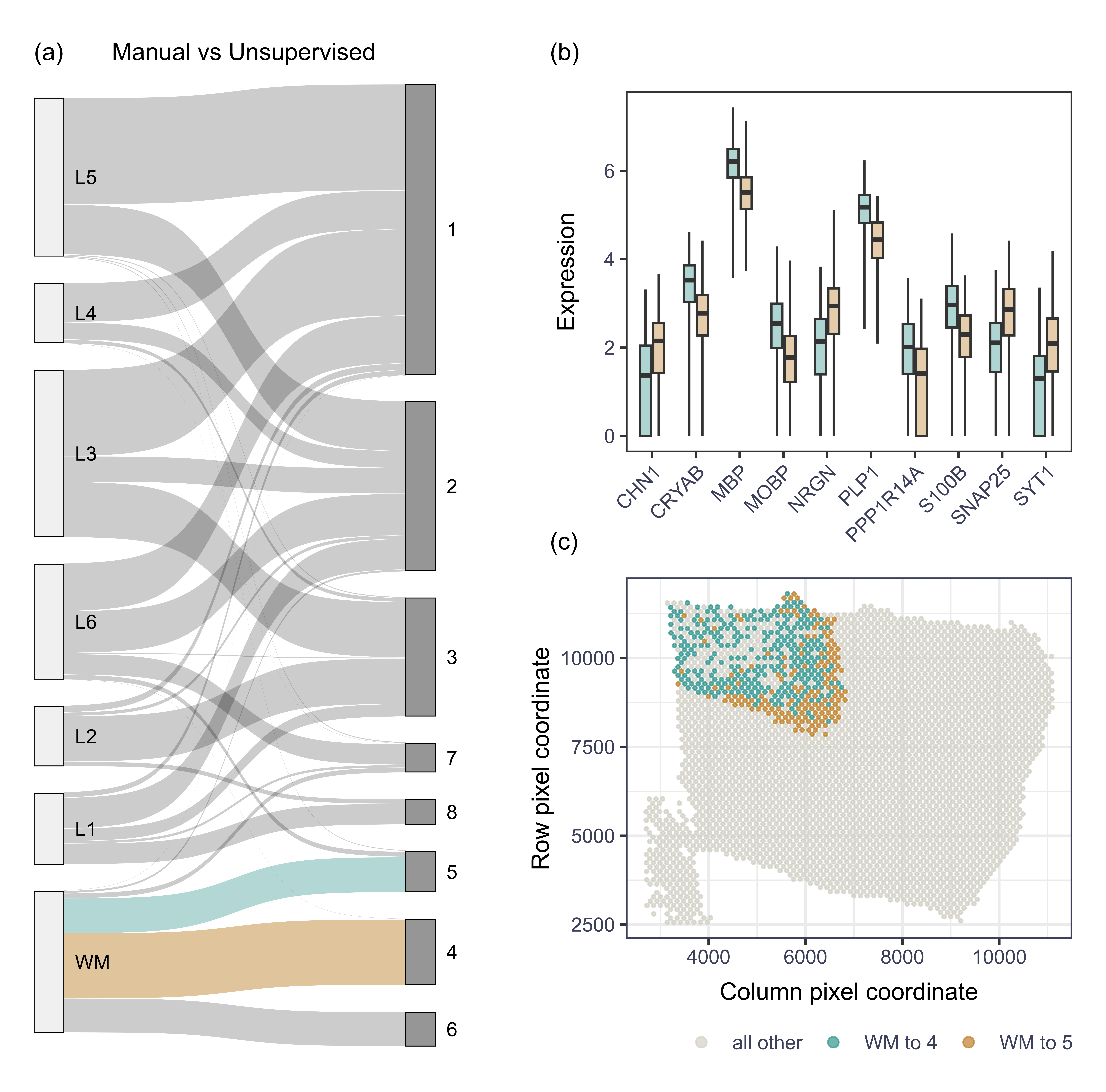al., 2021). Figure 1 explores the comparison between spots manually labelled as White Matter (WM) but annotated as two different clusters in the unsupervised approach. Notice that we used tagtango to filter out the results, focusing on one sample (i.e. labelled as 151675) excluding non-tissue spots (i.e. classified as NA in the manual annotations). This comparison identified key genes driving the distinction between sub-populations within the manually annotated WM region. These include known WM and L5 marker genes such as MBP, which, coupled with the fact that spots in cluster 4 did not intersect with spots manually labelled as L5 or L6, suggests additional modularity within the WM layer. Similarly, a marker gene for gray matter/neurons that was used to define the sample orientation by Maynard et. al., 2021, SNAP25 is also identified as relevant. Finally, MOBP, a gene identified as top 10th most variable markers across layers by the author but that our comparison suggests this also show some level of modularity within WM, was also selected as relevant.

Figure 1: Overview of the comparison between layer annotations in the brain cortex dataset. Panel (a) displays a Sankey diagram comparing the manual and unsupervised annotations. The diagram was filtered using tagtango to only include cells from sample `151675’ and in-tissue spots. The coloured links in the diagram indicate the cell populations selected for White Matter (WM). Panel (b) displays a direct comparison of the normalized RNA expression for the two selected cell populations, including only markers selected as relevant. The colours of the bars match those of the selected links in panel (a). Panel (c) presents the spatial representation of all spots, where the colours of the points match those of the selected links in panel (a).

Notice that there are multiple types of comparisons that could be performed with tagtango. For example, we could try to understand differences between the way the different co-authors of the study labelled the spots, annotations that are also provided with the R package. Likewise, we could focus on comparing full layers, reproducing the authors results and potentially identifying additional marker genes separating the cortex layers.

Supplementary usage scenario: understanding batch effects

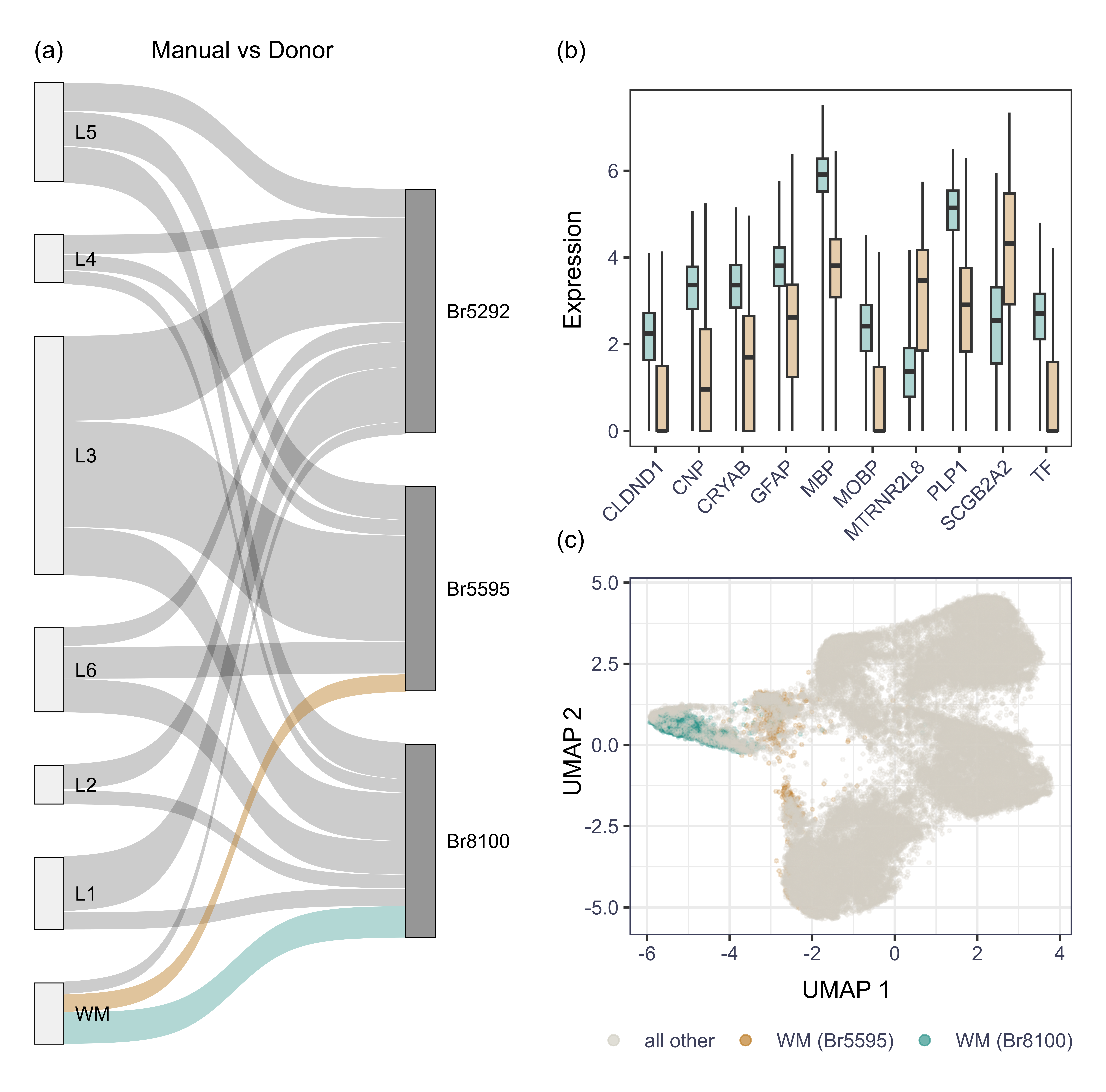
An interesting use case for tagtango is the identification of marker differences across batches. To illustrate this, we used the same spatial dataset described in the previous section to compare manually annotated brain layers to the donor IDs. Figure 2 explores the differences between WM in donors Br8100 and Br5595. In this case, we see strong differences in the normalized expression of several interesting genes. For example, we see large differences again for MBP, a marker gene that is central to the manual annotations. Likewise, we see batch effects in other notable genes such as CNP, identified by Zeng et. al., 2021 as brain cortex cell-type marker genes conserved between Human and Mouse. Finally, we see also differences for MOBP, highlighting this gene as not only variable across layers but also across batches.

Figure 2: Overview of the comparison between samples in the brain cortex dataset. Panel (a) displays a Sankey diagram comparing the manual annotations and donor ID. The diagram was filtered using tagtango to only include in-tissue spots. The coloured links in the diagram indicate the cell populations selected for deeper analysis. Panel (b) displays a direct comparison of the normalized RNA expression for the two selected cell populations, including only markers selected as relevant. The colours of the bars match those of the selected links in panel (a). Panel (c) presents the UMAP representation of the RNA expression for all spots, where the colours of the points match those of the selected links in panel (a).

Supplementary usage scenario: comparing single-cell datasets

As the final usage case scenario, we showcased how tagtango can be used to compare datasets. To do so, we used two independent 10x datasets: PBMCs from a healthy donor obtained by 10x Genomics from AllCells (10x Genomics, 2021), and PBMCs form a diseased Acute Lymphoblastic Leukemia donor obtained by 10x Genomics from Sanguine Biosciences (10x Genomics, 2024).

In order to analyse the datasets together with tagtango, we first independently processed and annotated each of them. To do so, we followed a three-step process: first, we downloaded the corresponding h5 file from the 10x Genomics platform; we then processed each dataset using the R packages Seurat (Hao et. al., 2023), SingleCellExperiment (Amezquita et. al., 2020) and scater (McCarthy et. al., 2017); and we use the R packages celldex and SingleR (Liu et. al., 2019) to annotate the single-cell datasets, identifying the main cell types. In R, the processing of each dataset is as follows:}

# Load libraries
library(Seurat)
library(SingleCellExperiment)
library(scater)
library(SingleR)
library(celldex)

# Set path to the h5 file downloaded from www.10xgenomics.com
path <- "path_to_h5_file"

# Load raw data
sce <- as.SingleCellExperiment(
       CreateSeuratObject(
            Seurat::Read10X_h5(path)
       )
 )

# calculate the proportion of mitochondrial reads
mt.genes <- rownames(sce)[grep("^MT-",rownames(sce))]
sce <- addPerCellQC(sce, subsets = list(Mito = mt.genes))

# perform QC
qc.lib <- isOutlier(sce$sum, log=TRUE, type="lower")
qc.nexprs <- isOutlier(sce$detected, log=TRUE, type="lower")
qc.mito <- isOutlier(sce$subsets_Mito_percent, type="higher")
sce$discard <- qc.lib | qc.nexprs | qc.mito
sce <- sce[,!sce$discard]

# Normalize counts
sce <- computeLibraryFactors(sce)
sce <- logNormCounts(sce)

# Annotate dataset with SingleR
ref <- BlueprintEncodeData()
pred <- SingleR(test=sce, ref=ref, labels=ref$label.main)
colData(sce) <- cbind(colData(sce), Main.labels = pred$labels)

This workflow provided us with two annotated SingleCellExperiment, one for the healthy patient (i.e.~sce\_healthy) and one for the cancer patient (i.e.~sce\_cancer). The last step before analysing the files with tagtango was to integrate these objects, removing biologically irrelevant batch effects. To do so, we used packages scran (Lun et. al., 2016) and batchelor (Haghverdi et. al., 2018) to correct the log-expression values via linear regression:

# Load libraries
library(scran)
library(batchelor)

# Find genes in common
universe <- intersect(rownames(sce_cancer_clean), rownames(sce_healthy_clean))

# Variance model
dec_cancer_clean <- modelGeneVarByPoisson(sce_cancer)[universe,]
dec_healthy_clean <- modelGeneVarByPoisson(sce_healthy)[universe,]

# Find HVGs
combined.dec <- combineVar(dec_cancer_clean, dec_healthy_clean)
chosen.hvgs <- combined.dec$bio > 0

# Per-batch scaling normalization
rescaled <- multiBatchNorm(sce_cancer[universe,], sce_healthy[universe,])
pbmc_cancer <- rescaled[[1]]
pbmc_healthy <- rescaled[[2]]

# Merge datasets and calculate TSNA
rescaled <- rescaleBatches(pbmc_cancer, pbmc_healthy)
rescaled <- runPCA(rescaled, subset_row=chosen.hvgs,
                 exprs_values="corrected",
                 BSPARAM=BiocSingular::RandomParam())
rescaled <- runTSNE(rescaled, dimred="PCA")

# Copy annotations and batch information
rescaled$batch <- factor(rescaled$batch, levels = c(1,2), labels = c("cancer", "healthy"))
rescaled$annotations <- c(pbmc_cancer$Main.labels, pbmc_healthy$Main.labels)

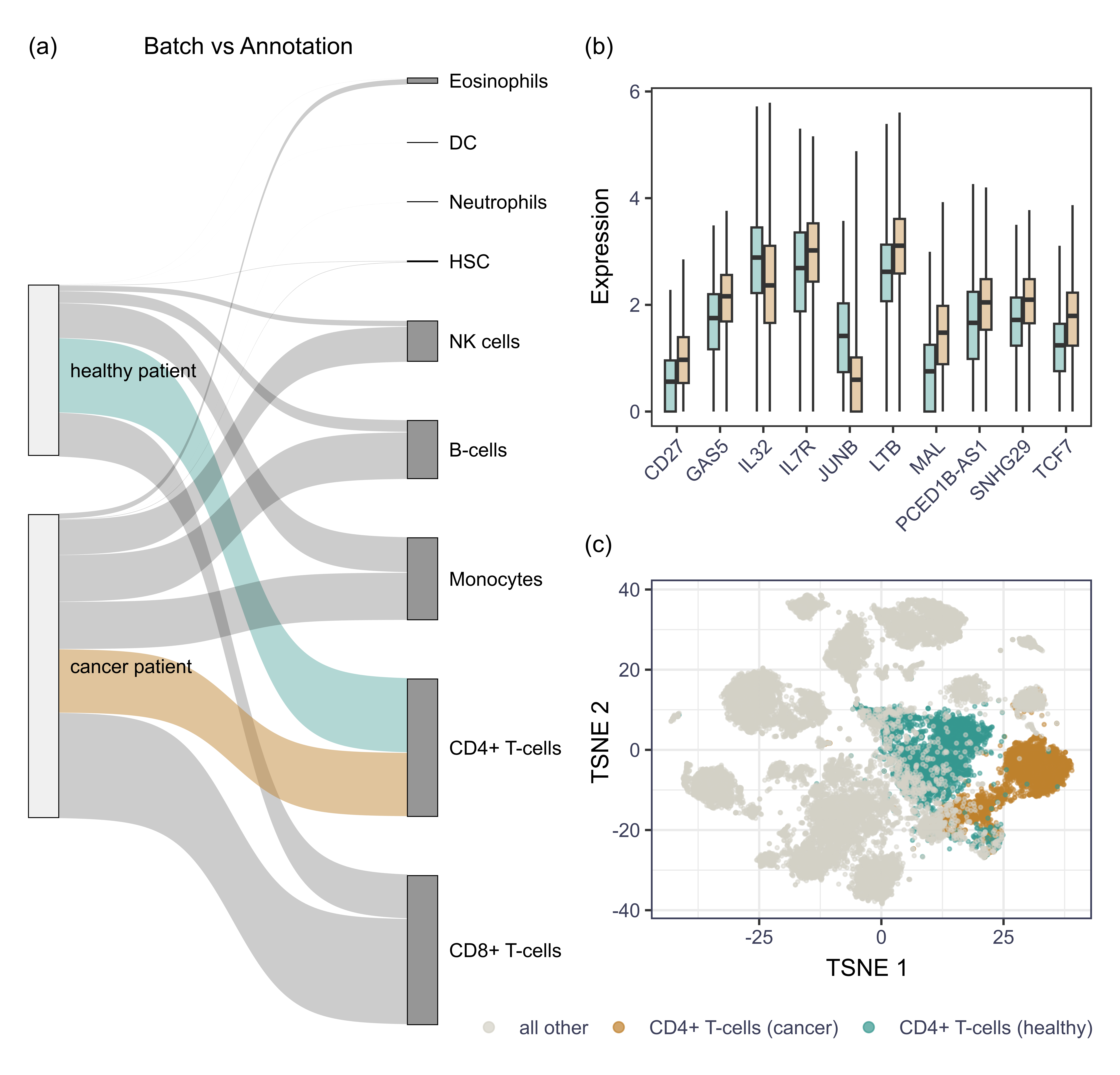
Using tagtango, we then compared the batch information and the annotations found with singleR (Figure 3). In particular, we focused on the differences across cells annotated as CD4+ T-cells across the two datasets. Again, tagtango highlighted differences in the normalized expression of several interesting genes, all related to immune response in cancer. Notably, JUNB has been identified in the past as a gatekeeper for a certain type of lymphoid leukemia (Ott et. al., 2007), and LTB has been shown to promote the development of T-cell acute lymphoblastic leukemia (Fernandes et. al., 2015). Likewise, genes such as CD27 or IL-32 have been closely associated to the clinical outcome and prognostic of acute lymphoblastic leukemia patients (Chen et. al., 2017; Abobakr et. al., 2023; Shim et. al., 2022), and there are links between the expression of IL-7R and TCF7 with subsets of these patients (Oliveira et. al., 2019; Van Thillo et. al., 2021). Overall, tagtango was able to quickly identify genes that are associated with lymphocyte development, transcriptional regulation, and immune signaling pathways in acute lymphoblastic leukemia patients. However, further work would be required to validate these findings and ensure their biological relevance.

Figure 3: Overview of the comparison between datasets using tagtango. Panel (a) displays a Sankey diagram comparing the batch information and main cell types. The coloured links in the diagram indicate the cell populations selected for deeper analysis. Panel (b) displays a direct comparison of the normalized and batch-corrected RNA expression for the two selected cell populations, including only markers selected as relevant. The colours of the bars match those of the selected links in panel (a). Panel (c) presents the TSNE representation of the RNA expression, where the colours of the points match those of the selected links in panel (a).